As much as R is popular in data analysis, R becomes more and more favored in geospatial analysis and visualization.
To introduce spatial data, let first start with comman data. Basic R data types: vector, factor, matrix, data.frame, and list.
Data and Plots
There are many ways to munipulate and visualize data in R, including, typically, the basic and the tidyverse framework. Let’s warm up with plotting data.frame.
basic plot
attach(mtcars)
par(mfrow = c(1,2))
plot(mpg, wt, main = "wt vs. mpg")
hist(mpg)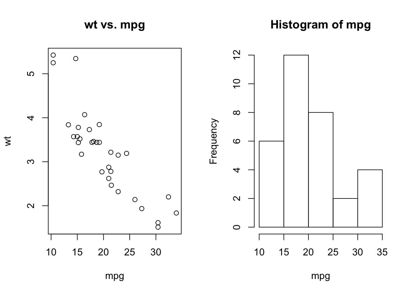
ggplot2
library(ggplot2)
p1  <- ggplot(mtcars, aes(x = mpg, y = wt)) +
  geom_point() +
  ggtitle("wt vs. mpg") +
  theme(plot.title = element_text(hjust = 0.5))
p2  <- ggplot(mtcars, aes(mpg)) +
  geom_histogram(binwidth = 5, color = 'black', fill = 'white') +
  ggtitle("mpg Histogram") +
  theme(plot.title = element_text(hjust = 0.5))
library(grid)
library(gridExtra)
grid.arrange(p1, p2, ncol = 2)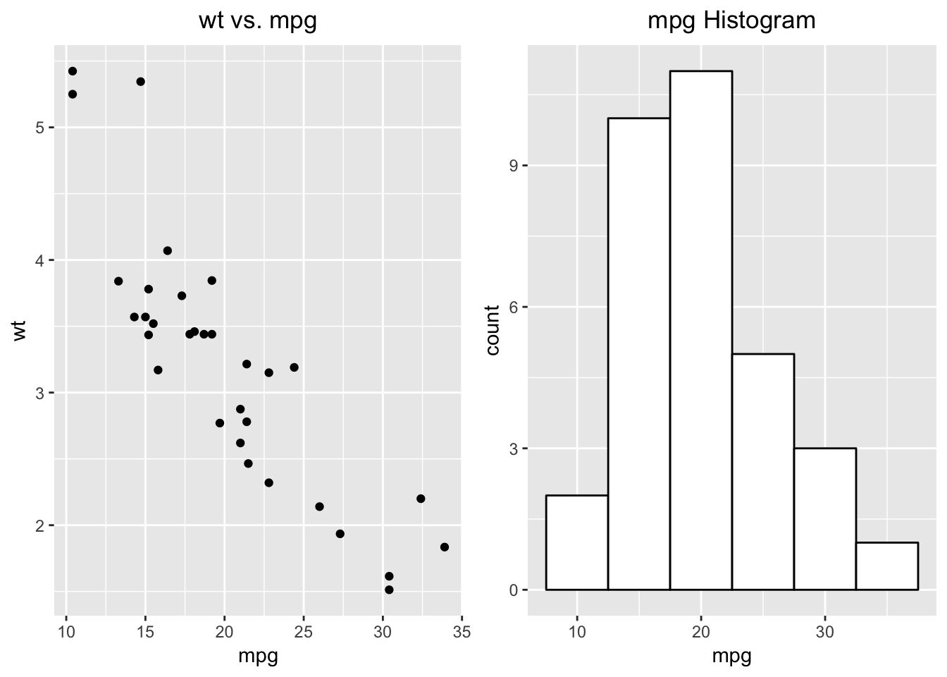
Spatial Data and Plots
# Load a csv file as data.frame as usual
dfUS <- read.csv("/Users/cxiao/Documents/Rmd/Station_US.csv")
# Take a look at the data.frame
head(dfUS)
## Num Station Lat Lon Avail
## 1 1 4074950 45.19133 -88.73779 1
## 2 2 4177720 41.52899 -84.88253 1
## 3 3 4077630 44.89831 -88.84534 1
## 4 4 4109000 42.29428 -84.40427 1
## 5 5 4178000 41.38407 -84.80254 1
## 6 6 4180988 40.70275 -84.65022 1# A bounch of USGS gages with lations
dfUS$Station <- paste0("0", dfUS$Station)How to transfer a data.frame to a spatial class?
First, get the coordinates
library(sp)
coords  <- SpatialPoints(dfUS[, c('Lon', 'Lat')])
Let’s check the above variable
class(coords)## [1] "SpatialPoints"
## attr(,"package")
## [1] "sp"str(coords)## Formal class 'SpatialPoints' [package "sp"] with 3 slots
## ..@ coords : num [1:392, 1:2] -88.7 -84.9 -88.8 -84.4 -84.8 ...
## .. ..- attr(*, "dimnames")=List of 2
## .. .. ..$ : NULL
## .. .. ..$ : chr [1:2] "Lon" "Lat"
## ..@ bbox : num [1:2, 1:2] -92.6 40.7 -74.5 47.5
## .. ..- attr(*, "dimnames")=List of 2
## .. .. ..$ : chr [1:2] "Lon" "Lat"
## .. .. ..$ : chr [1:2] "min" "max"
## ..@ proj4string:Formal class 'CRS' [package "sp"] with 1 slot
## .. .. ..@ projargs: chr NAhead(coords)## SpatialPoints:
## Lon Lat
## [1,] -88.73779 45.19133
## [2,] -84.88253 41.52899
## [3,] -88.84534 44.89831
## [4,] -84.40427 42.29428
## [5,] -84.80254 41.38407
## [6,] -84.65022 40.70275
## Coordinate Reference System (CRS) arguments: NAWe can see, it’s a SpatialPoints class, looking like data.frame, only with coordinates but with any meaningful data.
Second, assign data to the SpatialPoints
spUS  <- SpatialPointsDataFrame(coords, dfUS)
# Check the new variable
class(spUS)
## [1] "SpatialPointsDataFrame"
## attr(,"package")
## [1] "sp"str(spUS)## Formal class 'SpatialPointsDataFrame' [package "sp"] with 5 slots
## ..@ data :'data.frame': 392 obs. of 5 variables:
## .. ..$ Num : int [1:392] 1 2 3 4 5 6 7 8 9 10 ...
## .. ..$ Station: chr [1:392] "04074950" "04177720" "04077630" "04109000" ...
## .. ..$ Lat : num [1:392] 45.2 41.5 44.9 42.3 41.4 ...
## .. ..$ Lon : num [1:392] -88.7 -84.9 -88.8 -84.4 -84.8 ...
## .. ..$ Avail : int [1:392] 1 1 1 1 1 1 1 1 1 1 ...
## ..@ coords.nrs : num(0)
## ..@ coords : num [1:392, 1:2] -88.7 -84.9 -88.8 -84.4 -84.8 ...
## .. ..- attr(*, "dimnames")=List of 2
## .. .. ..$ : NULL
## .. .. ..$ : chr [1:2] "Lon" "Lat"
## ..@ bbox : num [1:2, 1:2] -92.6 40.7 -74.5 47.5
## .. ..- attr(*, "dimnames")=List of 2
## .. .. ..$ : chr [1:2] "Lon" "Lat"
## .. .. ..$ : chr [1:2] "min" "max"
## ..@ proj4string:Formal class 'CRS' [package "sp"] with 1 slot
## .. .. ..@ projargs: chr NAplot(spUS)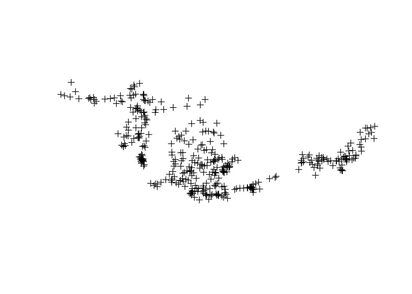
After tmap is loaded
library(tmap)
spUS
## class : SpatialPointsDataFrame
## features : 392
## extent : -92.63297, -74.54355, 40.70275, 47.48204 (xmin, xmax, ymin, ymax)
## coord. ref. : NA
## variables : 5
## names : Num, Station, Lat, Lon, Avail
## min values : 1, 04015330, 40.70275, -74.54355, 0
## max values : 392, 0441624088045601, 47.48204, -92.63297, 1A Spatial class variable will not be entirely dumped out.
# try tmap::qtm
qtm(spUS)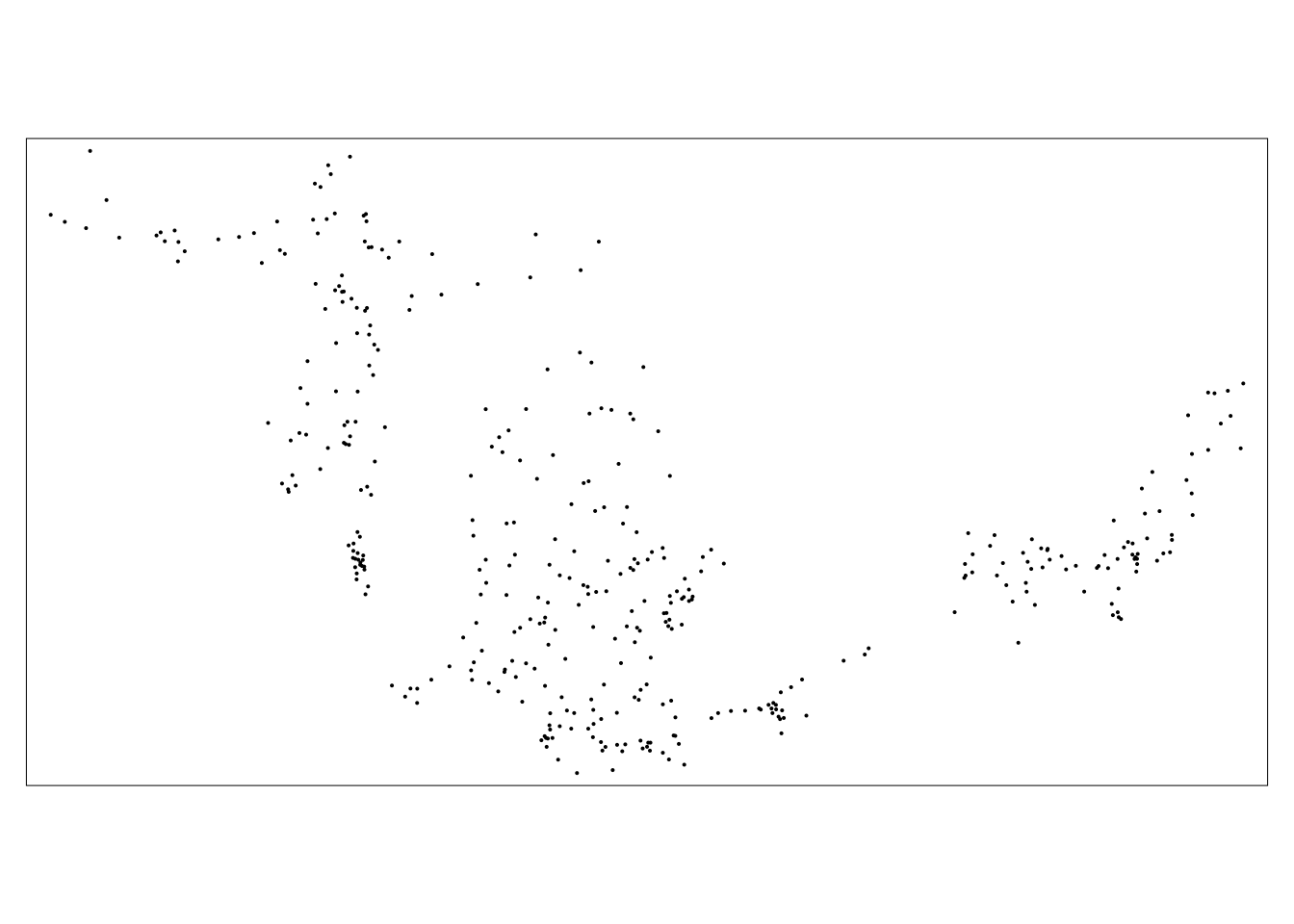
Difference between data.frame and SpatialPointsDataFrame
data.frameuses$to access its columns.- e.g.
dfUS$Station
- e.g.
SpatialPointsDataFrameuses@to access its four lists:data,coords.nrs,coords,bboxandproj4string; while$to itsdatacolumns.- e.g.
spUS@data, thenspUS@data$Station, or simplyspUS$Station
- e.g.
Another quick way
pnt1  <- dfUS
coordinates(pnt1) = ~ Lon + Lat
Shape objects
| Without data | With data | |
|---|---|---|
| Polygons | SpatialPolygons | SpatialPolygonsDataFrame |
| Points | SpatialPoints | SpatialPointsDataFrame |
| Lines | SpatialLines | SpatialLinesDataFrame |
| Raster | SpatialGrid | SpatialGridDataFrame |
| Raster | SpatialPixels | SpatialPixelsDataFrame |
| Raster | RasterLayer | |
| Raster | RasterBrick | |
| Raster | RasterStack |
Reading
- Tutorial: Creating maps in R by Robin Lovelance and James Cheshire
- website r-spaital.org by Edzer Pebesma
- CRAN Task View: Analysis of Spatial Data by Roger Bivand
Packages
rgdal: R’s interface to Geospatial Data Abstraction Library (GDAL)rgdal::readOGR, to read OGR vector maps (e.g. shapfile) into Spatial objects
rgeos: R’s interface to the powerful vector processing library geos
maptools: provides various mapping functions
tmap: a new packages for rapidly creating beautiful maps- An extenstion wrap of the basic
plot qtm, quick thematic map plot
tm_shape,tm_fill
- An extenstion wrap of the basic
ggmap: extends the plotting packageggplot2for maps- add a variaty of basemaps
leaflet: interactive map from its JavaScript
mapview: interactive viewing spatial data based onleaflet
maptools::readShapeSpatial
The use of
maptools::readShapeSpatialhas been deprecated. Usergdal::readOGRandsf::st_readinstead.