zoo: S3 Infrastructure for Regular and Irregular Time Series (Z’s Ordered Observations)
An S3 class with methods for totally ordered indexed observations. It is particularly aimed at irregular time series of numeric vectors/matrices and factors. zoo’s key design goals are independence of a particular index/date/time class and consistency with ts and base R by providing methods to extend standard generics
Base Time-Series Objects stats::ts
Credit: Time Series Analysis in R Part 1: The Time Series Object by DataSciencePlus
From the base
tsobjects to a whole host of other packages likexts,zoo,TTR,forecast,quantmodandtidyquant, R has a large infrastructure supporting time series analysis.
Monthly/Quaterly TS
ts1 <- ts(1:10, frequency = 12, start = c(1959, 2)) # Feburary of 1959
ts1; class(ts1)
## Feb Mar Apr May Jun Jul Aug Sep Oct Nov
## 1959 1 2 3 4 5 6 7 8 9 10## [1] "ts"ts2 <- ts(1:10, frequency = 4, start = c(1959, 2)) # 2nd Quarter of 1959
ts2## Qtr1 Qtr2 Qtr3 Qtr4
## 1959 1 2 3
## 1960 4 5 6 7
## 1961 8 9 10Period TS
ts3 <- ts(1:10, frequency = 7, start = c(2012, 2))
print(ts3, calendar = TRUE)
## p1 p2 p3 p4 p5 p6 p7
## 2012 1 2 3 4 5 6
## 2013 7 8 9 10Plot TS
gnp <- ts(cumsum(1 + round(rnorm(100), 2)),
          start = c(1954, 7), frequency = 12)
plot(gnp) # using 'plot.ts' for time-series plot
zoo class
Read vector with a time index
library(zoo)
f1 <- system.file('doc/demo1.txt', package = 'zoo')
system(paste0("head ", f1))
inrusd <- read.zoo(f1, sep = "|", format="%d %b %Y")
class(inrusd)
## [1] "zoo"str(inrusd)## 'zoo' series from 2005-02-10 to 2005-03-10
## Data: num [1:20] 43.8 43.8 43.7 43.8 43.8 ...
## Index: Date[1:20], format: "2005-02-10" "2005-02-11" "2005-02-14" "2005-02-15" "2005-02-16" ...head(inrusd)## 2005-02-10 2005-02-11 2005-02-14 2005-02-15 2005-02-16 2005-02-17
## 43.78 43.79 43.72 43.76 43.82 43.74Read matrix with a time index
f2 <- system.file('doc/demo2.txt', package = 'zoo')
tmp <- read.table(f2, sep = ",")
z <- zoo(tmp[, 3:4], as.Date(as.character(tmp[, 2]), format="%d %b %Y"))
colnames(z) <- c("Nifty", "Junior")

head(z)
## Nifty Junior
## 2005-02-10 2063.35 4379.20
## 2005-02-11 2082.05 4382.90
## 2005-02-14 2098.25 4391.15
## 2005-02-15 2089.95 4367.25
## 2005-02-17 2061.90 4320.15
## 2005-02-18 2055.55 4318.15Convert back to matrix
plain1 <- coredata(z)
head(plain1)
## Nifty Junior
## [1,] 2063.35 4379.20
## [2,] 2082.05 4382.90
## [3,] 2098.25 4391.15
## [4,] 2089.95 4367.25
## [5,] 2061.90 4320.15
## [6,] 2055.55 4318.15# with rownames
plain2 <- as.matrix(z)
head(plain2)## Nifty Junior
## 2005-02-10 2063.35 4379.20
## 2005-02-11 2082.05 4382.90
## 2005-02-14 2098.25 4391.15
## 2005-02-15 2089.95 4367.25
## 2005-02-17 2061.90 4320.15
## 2005-02-18 2055.55 4318.15Selecting (subsetting)
window(z, start = as.Date("2005-02-15"), end = as.Date("2005-02-28"))## Nifty Junior
## 2005-02-15 2089.95 4367.25
## 2005-02-17 2061.90 4320.15
## 2005-02-18 2055.55 4318.15
## 2005-02-21 2043.20 4262.25
## 2005-02-22 2058.40 4326.10
## 2005-02-23 2057.10 4346.00
## 2005-02-24 2055.30 4337.00
## 2005-02-25 2060.90 4305.75
## 2005-02-28 2103.25 4388.20z[as.Date("2005-03-10")]## Nifty Junior
## 2005-03-10 2167.4 4648.05Missing Value
# only rows with data from both x and y are included in the output
m1 <- merge(inrusd, z, all = FALSE)
plot(m1)
# then extra rows will be added to the output with missing values
m2 <- merge(inrusd, z)
plot(m2)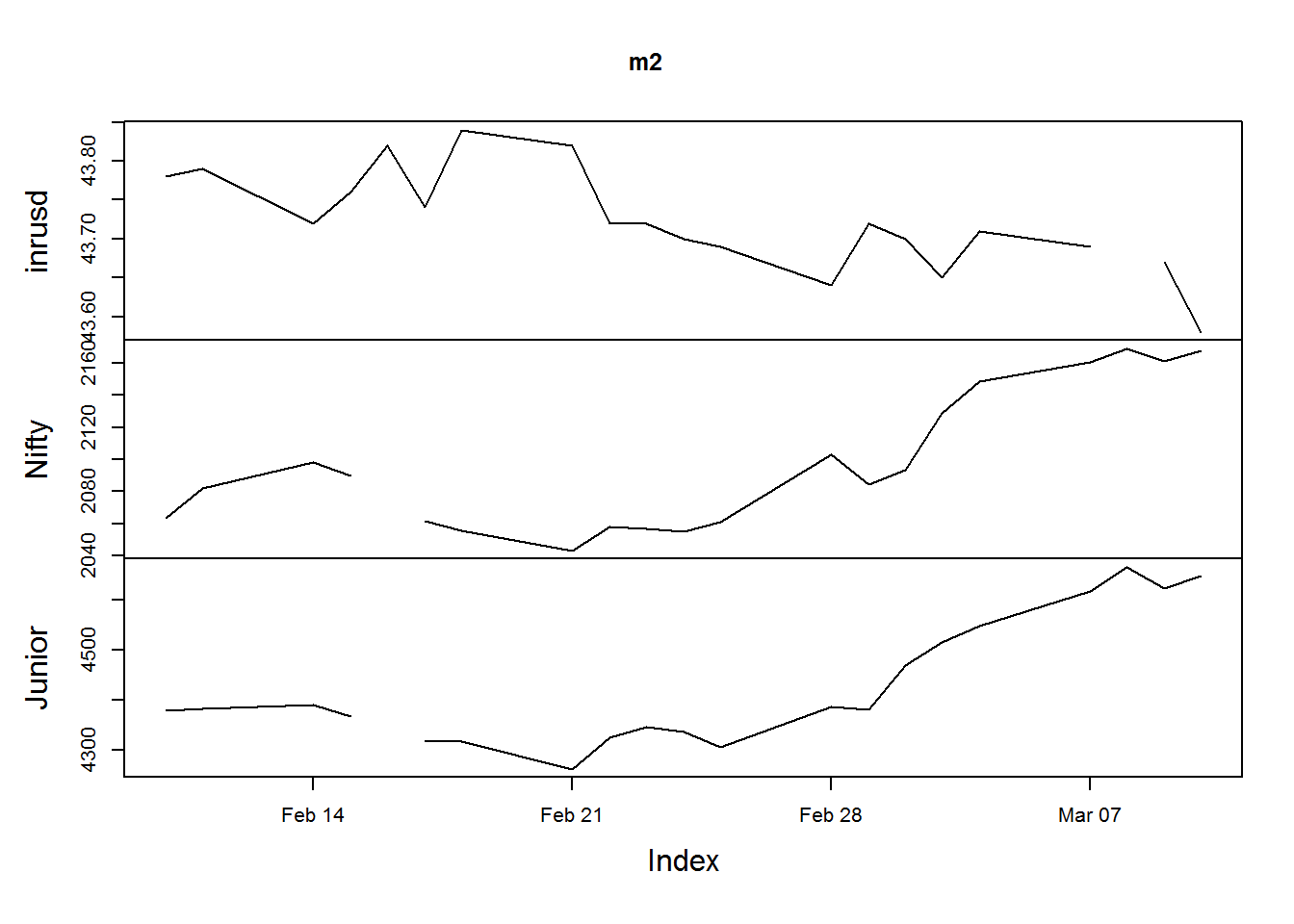
m_approx <- na.approx(m2)# Replaced by linear interpolation via approx
m_locf   <- na.locf(m2)  # Last Observation Carried Forward
Plot
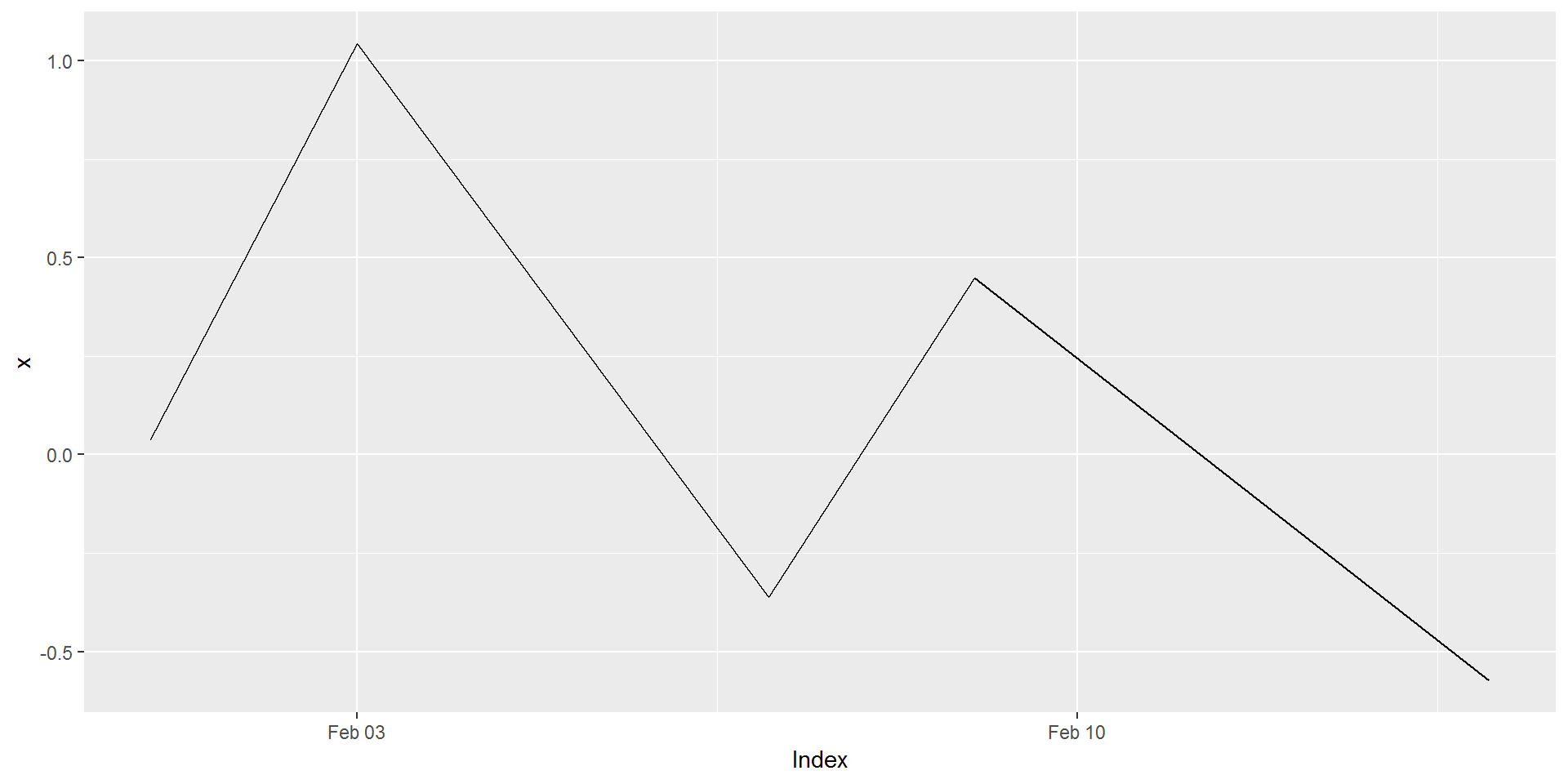
library(ggplot2)## Warning: package 'ggplot2' was built under R version 3.5.1x.Date <- as.Date(paste(2003, 02, c(1, 3, 7, 9, 14), sep = "-"))
x <- zoo(rnorm(5), x.Date)
xlow <- x - runif(5)
xhigh <- x + runif(5)
#z <- cbind(x, xlow, xhigh)
## univariate plotting
## calling ggplot2.zoo
## autoplot(x)
## broom zoo to data.frame
ggplot(aes(x = index, y = value), data = broom::tidy(x)) +
geom_line() + xlab("Index") + ylab("x")